Optimizing Decision Trees: How to Calculate Splits with Gini Impurity
By Mbali Kalirane on
Gini impurity quantifies the uncertainty in a data set by measuring the probability of incorrectly classifying a data point based on the distribution of labels in the subset. Calculating the Gini impurity for each feature helps identify which feature results in the lowest impurity and hence maximizes the homogeneity of the resulting child nodes. This process of calculating Gini impurity helps us choose the most informative features for partitioning our dataset.
In this article, we’ll go through an example of how to use gini impurity for effectively partitioning data in a decision tree.
Table of Contents
Steps for Splitting a Decision Tree
1. Calculate the Gini impurity for each feature subcategory
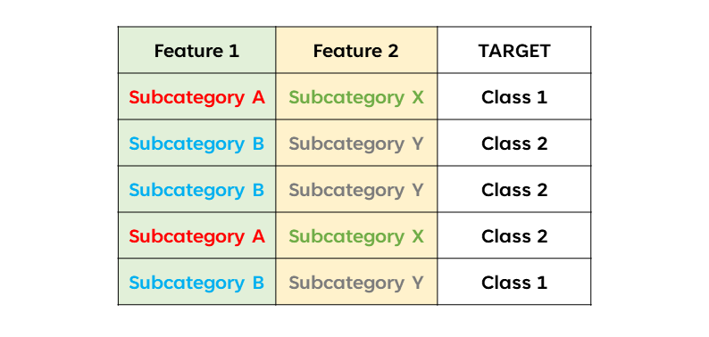
Suppose we have the following hypothetical dataset, with two independent variables, Feature 1, Feature 2, and a target variable, Target. Feature 1 has two subcategories, A and B. Feature 2 has subcategories, X an Y. The target variables have two classes, class 1 and class 2.
We calculate the Gini of each feature’s subcategory as follows:
\(Gini(subcategory) = 1 - \sum_{i=1}^{n} p(subcategory \mid Class_i)^2\),
What we’re doing is we’re calculating the sum of the probabilities of an instance belonging to a specific subcategory, given that it belongs to each Target class, $Class_i$.
For example, for Feature 1 we have two subcategories A and B. Thus, we’d calculate the gini impurity for both subcategories as follows:
\[Gini(A) = 1 - (p(\text(A | Class 1))^2 + p(\text(A | Class 2)))^2\] \[Gini(B) = 1 - (p(\text(B | Class 1))^2 + p(\text(B | Class 2)))^2\]We’d do the same for Feature 2.
2. Calculate the weighted Gini impurity for each feature:
The weighted gini is a combination of the Gini impurities of the subcategories in each Feature . In other words, it’s a combination of the gini impurities of the left branch and the gini of the right branch of the decision tree. It involves multiplying of the probability of each Feature with the gini of the feature and is calculated as follows:
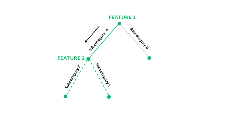
\[G_{\text{weighted}} = \frac{N_{\text{left}}}{N_{\text{total}}} G_{\text{left}} + \frac{N_{\text{right}}}{N_{\text{total}}} G_{\text{right}}\]When splitting a feature, each subcategory in that feature corresponds to a branch in the decision tree. For example, in the below decision tree, Feature 1 has branches, A and B, which correspond to subcategories A and B.
Thus, for Feature 1, we’d calculate the gini impurity by combining the Gini impurities for branches (subcategories) A and B as follows:
\[Gini(\text{Feature 1}) = p(A)Gini(A) + p(B)Gini(B)\]We’d apply the same process for calculating the weighted gini the for other features in the dataset.
3. Choose the feature with the lowest Gini impurity as the root node
Let’s assume that $Gini(\text{Feature 1})$ is smaller than $Gini(\text{Feature 2})$. Thus, we’d choose Feature 1 as our root node.
4. Calculate the subnodes, considering the branches of the previous node
Since we’ve chosen our root node to be “Feature 1”, we have two possible branches where our subnode will be located. These are branches A and B. If our subnode is located on branch A, we consider branch A when calculating the gini impurity of our subnode. Essentially, we calculate the Gini impurity of Feature 2, given that it’s in branch A:
\[Gini(\text{Feature 1|Branch A})\]An Example of Calculating Gini Impurity
Let’s assume we have a dataset with two features, “color” and “size”, and a target variable, “buy”, signifying an item being bought (yes or no) depending on the features “color” and “size”. The “color” feature has subcategories, “red” and “blue”. And “size” has subcategories, “small” and “large”.
\[\begin{array}{|c|c|c|} \hline \text{Color} & \text{Size} & \text{Buy} \\ \hline \text{Red} & \text{Small} & \text{Yes} \\ \hline \text{Red} & \text{Large} &\text{No} \\ \hline \text{Blue} & \text{Small} & \text{Yes} \\ \hline \text{Blue} & \text{Large} & \text{No} \\ \hline \text{Red} & \text{Small} & \text{No} \\ \hline \end{array}\]Calculating the Root Node of a Decision Tree
For each feature in the dataset, we first calculate the gini impurity of each feature’s subcategories, and then calculate the weighted (combined) gini impurity for that feature.
1. For the Color Feature
The color feature has subcategories, “red” and “blue”. We’ll first calculate the Gini impurity for the “Red” subcategory and then the Gini for the “Blue” subcategory. Finally, we’ll calculate the weighted Gini of the Color feature, by combining the Gini impurities of the “blue” and “red” subcategories.
RED Subcategory
The probability that the item is red:
$P(Red) = \frac{3}{5}$
The probability of the item being red, given that it’s in the class “yes”:
$P(Red_{yes}) = \frac{1}{3}$
The probability of the item being red, given that it’s in the class “no”:
$P(Red_{no}) = \frac{2}{3}$
The gini impurity for the “red” class:
$Gini(Red) = 1 - P(Red_{yes})^2 - P(Red_{no})^2$
$= 1 - \frac{3}{5}^2 - \frac{2}{3}^2 = \frac{4}{9}$
BLUE Subcategory
Calculating for the “blue” subcategory:
The probability of the item being blue:
$P(Blue) = \frac{2}{5}$
The probability of the item being blue, given that it’s in the class “yes”:
$P(Blue_{yes}) = \frac{1}{2}$
The probability of the item being red, given that it’s in the class “no”:
$P(Blue_{no}) = \frac{1}{2}$
The gini of the blue class:
$Gini(Blue) = 1 - P(Blue_{yes})^2 - P(Blue_{no})^2$
$= 1 - \frac{1}{2}^2 - \frac{1}{2}^2 = \frac{1}{2}$
Weighted Gini for Color Feature:
$Gini(Color) = P(Red)Gini(Red)+P(Blue)Gini(Blue)$
$= \frac{3}{5}(\frac{4}{9}) + \frac{2}{5}(\frac{1}{2}) = \frac{7}{15}$
Size Feature
The size features has subcategories, “small” and “large”. We’ll first calculate the Gini impurity for the “Small” subcategory and then the Gini for the “Large” subcategory. Finally, we’ll calculate the weighted Gini of the Size feature, by combining the Gini indexes of the “small” and “large” subcategories.
SMALL Subcategory
The probability of the item being small:
$P(Small) = \frac{3}{5}$
The probability of the item being small, given that it’s in the class “yes”:
$P(Small_{yes}) = \frac{2}{3}$
The probability of the item being small, given that it’s in the class “no”:
$P(Small_{no}) = \frac{1}{3}$
The gini for the small class:
$Gini(Small) = 1 - P(Small_{yes})^2 - P(Small_{no})^2$
$= 1 - \frac{2}{3}^2 - \frac{1}{3}^2 = \frac{4}{9}$
LARGE Subcategory
Calculating for the “large” subcategory:
The probability of the item being large:
$P(Large) = \frac{2}{5}$
The probability of the item being large, given that it’s in the class “yes”:
$P(Large_{yes}) = 0
The probability of the item being large, given that it’s in the class “no”:
$P(Large_{no}) = \frac{2}{2} = 1$
The gini for the Large class:
$Gini(Large) = 1 - P(Large_{yes})^2 - P(Large_{no})^2$
$= 1 - 0^2 - 1^2 = 0$
Weighted Gini for Size Feature:
$Gini(Size) = P(Small)Gini(Small)+P(Large)Gini(Large)$
$= \frac{3}{5}(\frac{4}{9}) + \frac{2}{5}(0) = \frac{4}{15}$
Choosing the Root Node of a Decision Tree
We’ll now choose the best starting feature for our decision tree. To do this, we choose the feature with the lowest gini impurity.
$Gini(Size) = \frac{4}{15}$
$Gini(Color) = \frac{7}{15}$
$\frac{4}{15} \leq \frac{7}{15}$.
“Size” feature has a smaller gini impurity than the “color” feature. Thus, our initial root node will be “size”.
Calculating the Sub Nodes of a Decision Tree
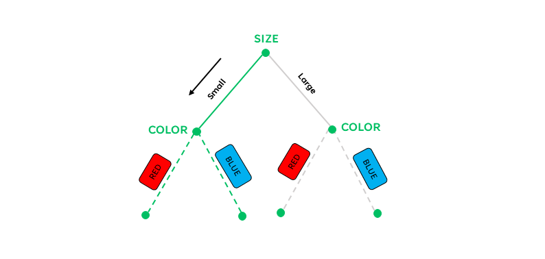
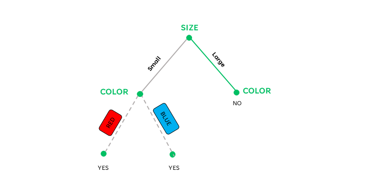
We’ll calculate the subnodes, by taking the into consideration the branches of the previous node. For example, consider this decision tree:
The “size” root node has two possible branches. These are “small” or “large”. The subnodes will occur at the end of these branches.
For the subnode on the “small” branch of the “size” feature, we’ll calculate for the gini impurity of the color feature, given that the size is small. For the subnode on the “large” branch of the “size” feature, we’ll calculate for the gini impurity of the color feature, given that the size is large.
For the Small Branch
We’ll calculate the Gini impurity for an item that’s red, given that its size is small. We’ll then calculate the Gini for an item that’s blue, given that its size is small” subcategory. Finally, we’ll calculate the weighted Gini of the “color” feature, given that the size is small.
RED given SMALL
The probability of the item being red given that it small:
$P(Red | Small) = \frac{2}{3}$
The probability of the item being small and red, given that it’s in the class “yes”:
$P(\text{Small and Red}_{yes}) = \frac{1}{2}$
The probability of the item being small and red, given that it’s in the class “no”:
$P(\text{Small and Red}_{no}) = \frac{1}{2}$
The gini of an item being red, given that it’s small:
\[Gini(\text{red | small}) = 1 - P(\text{Small and Red}_{yes})^2 - P(\text{Small and Red}_{no})^2\]$= 1 - \frac{1}{2}^2 - \frac{1}{2}^2 = \frac{1}{2}$
BLUE given SMALL
The probability of the item being blue given that it’s small:
$P(Blue | Small) = \frac{1}{3}$
The probability of the item being small and blue, given that it’s in the class “yes”:
$P(\text{Small and Blue}_{yes}) = 1$
The probability of the item being small and blue, given that it’s in the class “no”.
$P(\text{Small and Blue}_{no}) = 0$
Gini for Blue given Small:
\[Gini(\text{blue | small}) = 1 - P(\text{Small and Blue}_{yes})^2 - P(\text{Small and Blue}_{no})^2\]$= 1 - 1^2 - 0^2 = 0$
Weighted Gini for Small Feature:
\[Gini(Color | Small) = P(\text{red | small})Gini(\text{red | small})+P(\text{blue | small})Gini(\text{blue |small})\]$= \frac{2}{3}(\frac{1}{2}) + \frac{1}{3}(0) = \frac{1}{3}$
For the Large Branch
We’ll calculate the Gini impurity for a red item, given that its size is large. We’ll then calculate the Gini for a blue item, given that its size is large” subcategory. Finally, we’ll calculate the weighted Gini of the “color” feature, given that the size is large.
RED given LARGE
The probability of the item being red, given that it’s large:
$P(red | large) = \frac{1}{2}$
The probability of the item being large and red, given that it’s in the class “yes”:
$P(\text{Large and Red}_{yes}) = 0$
The probability of the item being large and red, given that it’s in the class “no”:
$P(\text{Large and Red}_{no}) = 1$
Gini impurity a red item, given that it’s large:
\[Gini(\text{red | large}) = 1 - P(\text{Large and Red}_{yes})^2 - P(\text{Large and Red}_{no})^2\]$= 1 - 0^2 - 1^2 = 0$
BLUE given LARGE
The probability of an item being blue, given that it’s large:
$P(blue | large) = \frac{1}{2}$
The probability of the item being large and blue, given that it’s in the class “yes”:
$P(\text{Large and Blue}_{yes}) = 0$
The probability of the item being large and blue, given that it’s in the class “no”:
$P(\text{Large and Blue}_{no}) = 1$
Gini of a blue item, given that it’s large:
\[Gini(\text{blue | large}) = 1 - P(\text{Large and Blue}_{yes})^2 - P(\text{Large and Blue}_{no})^2\]$= 1 - 0^2 - 1^2 = 0$
Weighted Gini for Large Feature:
\[Gini(Color | Large) = P(\text{red | large})Gini(\text{red | large})+P(\text{blue | large})Gini(\text{blue | large})\]$= \frac{1}{2}(0) + \frac{1}{2}(0) = 0$
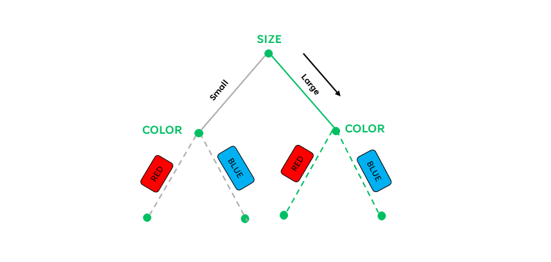
Since the Gini impurity for “large” is 0, no further splitting is required on this branch.
Thus, we have the following decision tree:
Conclusion
The process of calculating Gini Impurity for the root Node is as follows:
- Calculate Gini Impurity for the Root Node:
- $( Gini(node) = 1 - \sum_{i=1}^{n} (p_i)^2 )$, where $(p_i)$ is the proportion of samples belonging to class (i) in the node.
- Calculate Gini Impurity for Each Split:
- Iterate over each feature and its unique values.
- Calculate Gini Impurity for each split using the weighted sum of child node impurities.
- Select the split with the lowest Gini Impurity.
- Repeat the Process Recursively:
- After selecting the best split, recursively build child nodes until a stopping criterion is met, for example, maximum depth, minimum samples in a node.
